Genomics Model
1. Introduction of the Layers
As discussed in the previous section, there are several types of neural network models, and selecting the appropriate model depends on your specific task. In this section, we will focus on the layers that form the structure of these models, rather than delving into the models themselves. In earlier notes, we have covered other essential elements, such as activation functions and optimizers. Here, we will concentrate solely on layers.
2. Foundational Layers
Neural network models are constructed from layers and activation functions. In other words, understanding the foundational layers enables you to build your own model or easily comprehend how other models function. Below, we will introduce the most fundamental layers, including their descriptions, typical positions in a network, and practical use cases, highlighting what each layer can learn and where it can be applied. Following that, we will discuss additional layers that have evolved from these foundational layers and explore their roles as the basis for various advanced models.
2.1. Fully Connected Layer (FC Layer)

- Description: A layer where every neuron is connected to all nodes in the previous layer, allowing the network to learn complex relationships between all input features.
- Typical Position: Hidden layers, output layer.
- Use Case:
- What it can learn: It can learn global patterns and relationships across all input features, making it good for combining information from different parts of the data.
- Practical applications: Used in tasks like predicting house prices (by learning relationships between features like size, location, and age) or classifying text sentiment (e.g., positive or negative reviews). In biology, it can be used to predict drug response based on gene expression data.
- Advantages:
- Highly flexible: Can learn any complex relationship between input features due to its fully connected structure.
- Versatile: Suitable for a wide range of tasks, from regression to classification, as it can combine information globally.
- Potential Issues:
- High computational cost: Since every neuron connects to all nodes in the previous layer, the number of parameters grows quadratically with the input and output sizes (e.g., for an input of 1000 nodes and an output of 500 nodes, there are 500,000 weights), leading to high memory usage and slow training.
- Overfitting: The large number of parameters allows the model to memorize the training data rather than generalize, especially when the training dataset is small or lacks diversity.
- Required Activation Functions:
- No specific requirement; commonly used with ReLU for hidden layers (to introduce non-linearity) or Softmax/Sigmoid for the output layer (for classification tasks).
- Tunable Parameters:
- Number of neurons: Determines the size of the layer (e.g., 128 neurons).
- Weight initialization: The method used to initialize weights (e.g., Xavier initialization).
- Bias: Whether to include a bias term for each neuron (usually enabled by default).
- Used in Models: Foundational in simple feedforward neural networks like Multi-Layer Perceptrons (MLPs) for tasks such as digit classification (e.g., MNIST dataset). Also used in the final layers of many deep learning models (e.g., VGG, ResNet) to combine features for classification or regression.
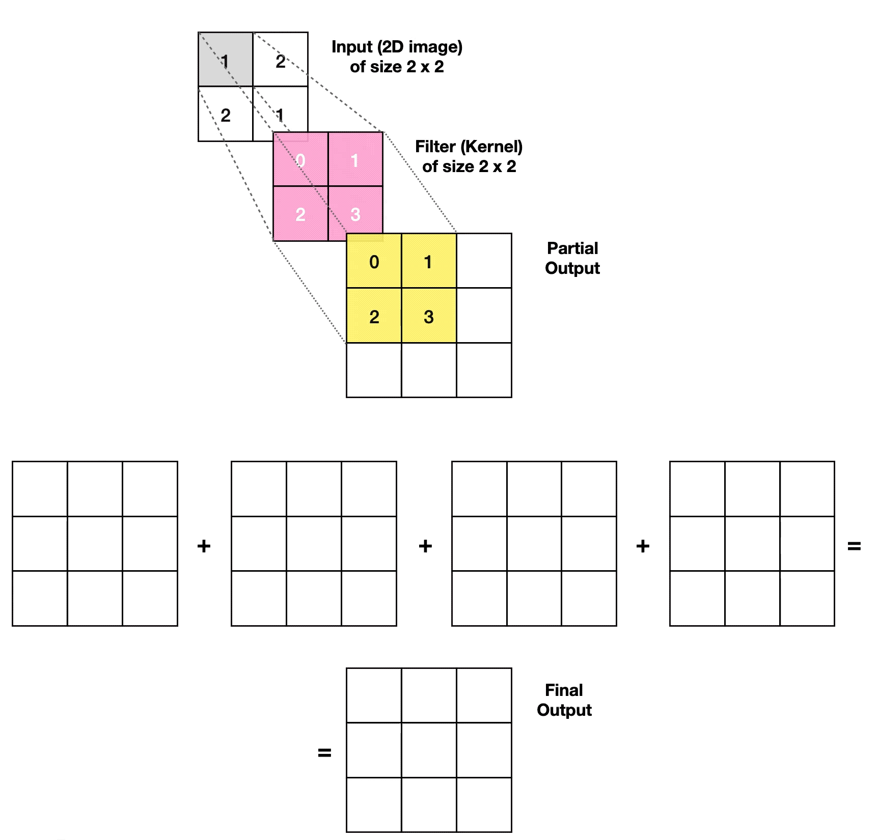
2.2. Convolutional Layer


- Article
- Description: A layer designed for grid-like data, such as images, that uses filters to detect local patterns like edges, textures, or shapes.
- Typical Position: Hidden layers.
- Use Case:
- What it can learn: It can learn local features in data, such as edges in images, patterns in time-series, or motifs in sequences.
- Practical applications: Commonly used in image recognition (e.g., identifying objects in photos, like cats or dogs) or video analysis (e.g., detecting actions in videos). In biology, it can detect patterns in DNA sequences for variant calling.
- Advantages:
- Parameter efficiency: Uses shared weights (filters), significantly reducing the number of parameters compared to a Fully Connected Layer.
- Translation invariance: Can detect patterns regardless of their position in the input, making it robust to shifts in data (e.g., an edge in an image).
- Potential Issues:
- Limited receptive field: Each filter only looks at a small local region (e.g., a 3x3 patch), so it cannot capture global relationships unless many layers are stacked, which increases computational cost and complexity.
- Sensitivity to input size: The output size depends on the input dimensions, stride, and padding; if the input size varies (e.g., images of different resolutions), the output size changes, which can cause issues in downstream layers expecting fixed sizes.
- Required Activation Functions:
- Typically used with ReLU to introduce non-linearity and help the network learn complex patterns.
- Tunable Parameters:
- Filter size: The size of the filter (e.g., 3x3 or 5x5).
- Number of filters: Determines how many feature maps are generated (e.g., 32 filters).
- Stride: The step size of the filter as it slides over the input (e.g., stride=1 or 2).
- Padding: Whether to add zeros around the input to preserve its size after convolution (e.g., “same” or “valid” padding).
- Dilation: The spacing between filter elements (e.g., dilation=1 for standard convolution, or higher for dilated convolution).
- Used in Models: Core component in Convolutional Neural Networks (CNNs) like AlexNet, VGG, ResNet, and Inception for image classification, object detection (e.g., YOLO), and semantic segmentation (e.g., U-Net). In biology, used in DeepBind for DNA sequence motif detection.
2.3. Recurrent Layer
- Description: A layer for sequential data, where it remembers past information to understand patterns over time or sequence.
- Typical Position: Hidden layers.
- Use Case:
- What it can learn: It can learn temporal or sequential dependencies, such as the order of words in a sentence or trends in a time-series.
- Practical applications: Used in language modeling (e.g., predicting the next word in a sentence) or speech recognition (e.g., transcribing audio to text). In biology, it can analyze time-series gene expression data to study how genes change over time.
- Advantages:
- Memory capability: Can remember past information, making it ideal for tasks where context or order matters (e.g., language or time-series).
- Sequential processing: Naturally handles data with a temporal or sequential structure, unlike other layers that treat inputs independently.
- Potential Issues:
- Gradient vanishing: Since all cells share the same weights and bias across time steps, during backpropagation through time (BPTT), gradients are repeatedly multiplied by the same weight matrix; if the weights are small, gradients shrink exponentially, making it hard to learn long-term dependencies.
- Gradient exploding: Similarly, if the shared weights are large, gradients can grow exponentially during BPTT, leading to unstable training (often mitigated by gradient clipping).
- Slow training: The sequential nature of processing (each time step depends on the previous one) prevents parallelization, so training cannot be sped up using GPUs as effectively as with other layers.
- Required Activation Functions:
- Typically used with Tanh as the default activation for hidden states, as it maps values to a range of [-1, 1], helping to stabilize training.
- Tunable Parameters:
- Hidden state size: The number of units in the hidden state (e.g., 128 units).
- Weight initialization: The method for initializing weights (e.g., orthogonal initialization).
- Return sequences: Whether to return the full sequence of outputs or just the final output (e.g., True or False).
- Direction: Whether the layer processes the sequence forward, backward, or both (e.g., bidirectional RNN).
- Used in Models: Foundational in early sequence models like vanilla RNNs for time-series prediction (e.g., stock price forecasting) and language modeling (e.g., ELMo). In biology, used in models like DeepSEA for predicting chromatin effects from genomic sequences.
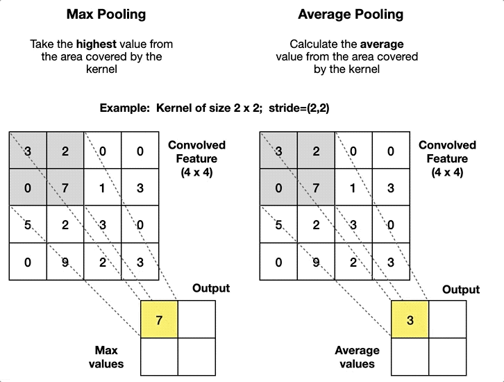
2.4. Pooling Layer
- Article
- Description: A layer that reduces the size of the data by summarizing regions, such as taking the maximum or average value in a small area.
- Typical Position: Hidden layers.
- Use Case:
- What it can learn: It can learn to focus on the most important features in a region, reducing noise and making the model more robust to small changes.
- Practical applications: Used in image processing to reduce image size while keeping key features (e.g., in facial recognition to focus on key facial features). In biology, it can reduce the dimensionality of genomic sequence data for easier processing.
- Advantages:
- Dimensionality reduction: Reduces the size of the data, lowering computational cost and memory usage.
- Robustness: Makes the model less sensitive to small shifts or distortions in the input by focusing on dominant features.
- Potential Issues and Why They Occur:
- Loss of information: The pooling operation (e.g., taking the maximum or average) discards all other values in the region, potentially losing fine-grained details that might be important for tasks requiring precise spatial information (e.g., pixel-level segmentation).
- Fixed operation: It applies a predefined rule (e.g., max or average) without learning, which may not be optimal for all tasks, as the best way to summarize features can vary depending on the data.
- Required Activation Functions:
- None; Pooling Layers do not use activation functions, as they perform a simple aggregation operation.
- Tunable Parameters:
- Pool size: The size of the window used for pooling (e.g., 2x2).
- Stride: The step size of the window as it slides over the input (e.g., stride=2).
- Type of pooling: The operation to apply (e.g., max pooling or average pooling).
- Padding: Whether to add zeros around the input to preserve its size (e.g., “same” or “valid” padding).
- Used in Models: Commonly used in CNNs like AlexNet, VGG, and ResNet to reduce spatial dimensions between convolutional layers, enabling efficient feature extraction. In biology, used in DeepVariant for reducing genomic data dimensions in variant calling.
3. Evolved Layers
The following layers have evolved from the foundational layers above, addressing specific limitations or extending their capabilities to handle more complex tasks. The layers are organized by their evolution paths, clarifying their dependencies (e.g., LSTM evolves from Recurrent Layer, and Attention Layer evolves from LSTM). Each evolved layer is described in terms of its origin, advantages, potential issues (with explanations of why they occur), required activation functions, tunable parameters, and its role as a foundational component in advanced models.
3.1. Evolution Path from Fully Connected Layer
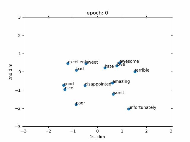
3.1.1. Embedding Layer
- Evolved From: Fully Connected Layer (used as a preprocessing step for discrete data).
- Description: Converts discrete data (like words or IDs) into continuous vectors, often used as an input to other layers like Fully Connected Layers.
- Advantages:
- Meaningful representations: Learns continuous vectors that capture similarities between discrete items (e.g., “king” and “queen” are close in vector space).
- Dimensionality reduction: Reduces the dimensionality of discrete data compared to one-hot encoding, making it more efficient.
- Potential Issues and Why They Occur:
- Fixed vocabulary: It relies on a predefined vocabulary (e.g., a fixed set of words), so new items not in the vocabulary cannot be embedded without retraining the embedding matrix.
- High dimensionality: For large vocabularies (e.g., 1 million words), the embedding matrix (vocabulary size × embedding dimension) becomes very large, increasing memory usage and computational cost.
- Required Activation Functions:
- None; Embedding Layers do not use activation functions, as they simply map indices to vectors.
- Tunable Parameters:
- Embedding dimension: The size of the continuous vectors (e.g., 300 dimensions).
- Vocabulary size: The number of unique items to embed (e.g., 10,000 words).
- Trainable: Whether the embeddings are fixed or trainable during training (e.g., True or False).
- Role in Models: A key component in models like Word2Vec and GloVe for word embeddings in NLP, and in recommendation systems (e.g., YouTube recommendation). In biology, used in models like DeepGO for gene function prediction by embedding gene IDs.
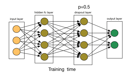
3.1.2. Dropout Layer
- Article
- Evolved From: Fully Connected Layer (as a regularization technique).
- Description: Randomly ignores some neurons during training to prevent the model from overfitting, initially applied to Fully Connected Layers.
- Advantages:
- Prevents overfitting: By randomly dropping neurons, it forces the network to learn more robust features.
- Simple to implement: Adds regularization with minimal computational overhead.
- Potential Issues and Why They Occur:
- Reduced capacity: Dropping neurons reduces the number of active units during training, which can limit the model’s ability to learn complex patterns, especially if the dropout rate is too high (e.g., 0.8).
- Inference difference: During inference, dropout is turned off, and all neurons are used, which can lead to a slight mismatch in behavior (e.g., the scale of outputs differs between training and testing).
- Required Activation Functions:
- None; Dropout Layers do not use activation functions, as they only modify the output of other layers.
- Tunable Parameters:
- Dropout rate: The probability of dropping a neuron (e.g., 0.5 means 50% of neurons are dropped).
- Role in Models: Used in a wide range of models, including AlexNet for image classification, BERT for NLP tasks, and LSTMs for sequence modeling, to improve generalization. In biology, used in DeepSEA to reduce overfitting in genomic sequence prediction.
3.1.3. Residual Connection
- Evolved From: Fully Connected Layer (as a structural improvement).
- Description: Adds a shortcut connection, allowing the network to learn differences (residuals) and train deeper networks more easily, initially applied to Fully Connected Layers.
- Advantages:
- Deeper networks: Allows training of very deep networks by mitigating gradient vanishing issues.
- Better optimization: Learning residuals is often easier than learning the full transformation, improving convergence.
- Potential Issues and Why They Occur:
- Increased complexity: Adds extra paths in the network (e.g., the shortcut connection alongside the main path), which can make debugging harder, especially in very deep networks with many residual connections.
- Not always beneficial: If the network is not deep enough (e.g., only a few layers), the benefits of residual connections are minimal, as gradient vanishing is less of an issue in shallow networks.
- Required Activation Functions:
- None; Residual Connections do not use activation functions, as they only add the input to the output.
- Tunable Parameters:
- None; Residual Connections are a structural modification and do not have tunable parameters (though the layers they connect may have parameters).
- Role in Models: Foundational in ResNet models for deep image classification (e.g., ResNet-50), and in deep language models like Transformer-XL. In biology, used in DeepVariant for high-dimensional genomic data analysis.
3.2. Evolution Path from Convolutional Layer
3.2.1. Transposed Convolutional Layer
- Article
- Evolved From: Convolutional Layer.
- Description: Increases the size of the data, often used to generate or upsample data like images, as an inverse operation to the Convolutional Layer.
- Advantages:
- Upsampling capability: Can generate or upsample data, making it ideal for tasks like image generation.
- Parameter efficiency: Like Convolutional Layers, it uses shared weights, keeping the number of parameters manageable.
- Potential Issues and Why They Occur:
- Checkerboard artifacts: The overlapping nature of transposed convolution (e.g., when stride > 1) can lead to uneven patterns in the output, as the filter applies weights in a grid-like manner, causing periodic artifacts.
- Limited control: It upsamples using a fixed filter pattern, which may not always produce semantically meaningful results, as it doesn’t learn the upsampling process adaptively.
- Required Activation Functions:
- Typically used with ReLU to introduce non-linearity, similar to Convolutional Layers.
- Tunable Parameters:
- Filter size: The size of the filter (e.g., 3x3). - Number of filters: Determines how many feature maps are generated (e.g., 32 filters).
- Stride: The step size for upsampling (e.g., stride=2).
- Padding: Whether to add zeros around the input (e.g., “same” or “valid” padding).
- Role in Models: Core to models like GANs (e.g., DCGAN) for image generation, U-Net for image segmentation, and super-resolution models (e.g., SRGAN). In biology, used in DeepChrome for upsampling chromosomal images.
3.2.2. Graph Convolutional Layer
The Graph Convolutional Layer extends the traditional Convolutional Layer to handle graph-structured data, such as social networks, knowledge graphs, or biological networks like protein-protein interaction (PPI) networks. Unlike images, which have a regular grid structure, graphs are irregular (non-Euclidean), with nodes (e.g., people, proteins) connected by edges (e.g., friendships, interactions). Graph Convolutional Layers learn by combining information from connected nodes, making them a core component of Graph Neural Networks (GNNs).
There are two main types of Graph Convolutional Layers: Spatial GCN and Spectral GCN. Both evolved from the Convolutional Layer but differ in how they process graph data. Below, we describe each type, highlighting their shared and unique characteristics.
Spatial Graph Convolutional Layer
(I couldn’t find a good tutorial video. Most of the videos are about spectral. If you know any good videos or article resources, please let me know.)
- Article, GitHub
- Evolved From: Convolutional Layer.
- Description: Spatial GCN processes graph data in the spatial domain, similar to how a Convolutional Layer processes images. It works by directly aggregating information from a node’s neighbors, mimicking how people in a social network might share information with their friends. For example, in a PPI network, a protein (node) updates its features by combining information from other proteins it interacts with (its neighbors).
- Advantages:
- Graph adaptability: Can handle irregular, non-Euclidean data like graphs, capturing relationships between nodes (e.g., friendships in a social network or interactions in a PPI network).
- Local aggregation: Efficiently combines information from neighboring nodes, similar to how Convolutional Layers focus on local patterns in images (e.g., edges in a photo). For instance, in a social network, a person’s interests might be influenced by their friends’ interests.
- Flexibility: Allows for various ways to combine neighbor information, such as summing, averaging, or using attention mechanisms to weigh the importance of different neighbors.
- Graph adaptability: Can handle irregular, non-Euclidean data like graphs, capturing relationships between nodes (e.g., friendships in a social network or interactions in a PPI network).
- Potential Issues and Why They Occur:
- Scalability: For large graphs, aggregating information from all neighbors can be computationally expensive. This is because the process involves iterating over all edges, which can be time-consuming in dense graphs with many connections (e.g., a social network where everyone is connected to many others).
- Over-smoothing: When stacking many layers, each layer aggregates information from neighbors, causing node features to become too similar over time. For example, in a deep GCN, a protein’s features might lose their uniqueness as they mix with features from distant proteins, reducing the model’s ability to distinguish between nodes.
- Scalability: For large graphs, aggregating information from all neighbors can be computationally expensive. This is because the process involves iterating over all edges, which can be time-consuming in dense graphs with many connections (e.g., a social network where everyone is connected to many others).
- Required Activation Functions:
- Typically uses ReLU to introduce non-linearity, just like Convolutional Layers in image processing. This helps the model learn complex patterns in the graph.
- Typically uses ReLU to introduce non-linearity, just like Convolutional Layers in image processing. This helps the model learn complex patterns in the graph.
- Tunable Parameters:
- Number of layers: The depth of the graph convolution (e.g., 2 layers), which determines how far information travels (e.g., a 2-layer GCN considers neighbors of neighbors).
- Aggregation method: How to combine neighbor information (e.g., summing, averaging, or attention-based methods like in Graph Attention Networks). This flexibility is unique to Spatial GCN.
- Dropout rate: The rate of dropout applied to node features to prevent overfitting (e.g., 0.5), ensuring the model doesn’t memorize the training data.
- Number of layers: The depth of the graph convolution (e.g., 2 layers), which determines how far information travels (e.g., a 2-layer GCN considers neighbors of neighbors).
- Role in Models: A key component of Graph Neural Networks (GNNs), used in models like GraphSAGE for large-scale node classification (e.g., user profiling in social networks) and Graph Attention Networks (GAT) for tasks requiring weighted neighbor contributions (e.g., knowledge graph reasoning). In biology, used in models like DeepGraphGO for predicting protein functions by analyzing PPI networks.
Spectral Graph Convolutional Layer
- Article
- Evolved From: Convolutional Layer.
- Description: Spectral GCN processes graph data in the spectral domain, using the mathematical properties of the graph’s structure. It’s like transforming a music signal into its frequencies (using a Fourier Transform) to analyze it, then transforming it back. Spectral GCN uses the graph’s Laplacian matrix—a mathematical representation of the graph’s structure—to define convolution, capturing global patterns in the graph. For example, in a PPI network, it might identify clusters of proteins that work together.
- Advantages:
- Graph adaptability: Like Spatial GCN, it can handle non-Euclidean data like graphs, capturing relationships between nodes (e.g., protein interactions in a biological network).
- Global structure sensitivity: Excels at capturing the overall structure of the graph, such as communities or functional modules. For instance, in a social network, it can identify groups of friends with similar interests, even if they’re not directly connected.
- Graph adaptability: Like Spatial GCN, it can handle non-Euclidean data like graphs, capturing relationships between nodes (e.g., protein interactions in a biological network).
- Potential Issues and Why They Occur:
- Scalability: Spectral GCN is even more computationally expensive than Spatial GCN for large graphs. It requires calculating the graph’s Laplacian matrix and performing matrix operations (e.g., matrix multiplications), which can be slow for dense graphs with many edges or large graphs with many nodes (e.g., a PPI network with thousands of proteins).
- Over-smoothing: Similar to Spatial GCN, stacking many layers causes node features to converge to similar values. In a deep Spectral GCN, the global mixing of features can make all proteins in a PPI network look too similar, losing their unique characteristics.
- Dependency on global structure: Spectral GCN relies on the entire graph’s structure, making it less suitable for dynamic graphs (e.g., a PPI network that changes under different conditions) because the Laplacian matrix must be recomputed whenever the graph changes.
- Scalability: Spectral GCN is even more computationally expensive than Spatial GCN for large graphs. It requires calculating the graph’s Laplacian matrix and performing matrix operations (e.g., matrix multiplications), which can be slow for dense graphs with many edges or large graphs with many nodes (e.g., a PPI network with thousands of proteins).
- Required Activation Functions:
- Typically uses ReLU to introduce non-linearity, similar to Spatial GCN and traditional Convolutional Layers.
- Typically uses ReLU to introduce non-linearity, similar to Spatial GCN and traditional Convolutional Layers.
- Tunable Parameters:
- Number of layers: The depth of the graph convolution (e.g., 2 layers), which affects how much global information is captured.
- Dropout rate: The rate of dropout applied to node features to prevent overfitting (e.g., 0.5). Unlike Spatial GCN, Spectral GCN does not have a tunable aggregation method, as its convolution is fixed by the spectral filter.
- Number of layers: The depth of the graph convolution (e.g., 2 layers), which affects how much global information is captured.
- Role in Models: A core component of Graph Neural Networks (GNNs), used in models like Kipf and Welling’s GCN for node classification (e.g., classifying research papers in citation networks like Cora) and ChebNet for graph signal processing. In biology, used in models like GraphProt for predicting protein-RNA interactions by identifying functional modules.
Key Differences
- Local vs. Global Focus: Spatial GCN focuses on local aggregation (like how CNNs focus on local patterns in images), while Spectral GCN captures global patterns using the graph’s spectral properties.
- Flexibility: Spatial GCN allows flexible aggregation methods (e.g., attention-based), while Spectral GCN’s convolution is fixed by its spectral filter.
- Scalability: Spectral GCN is generally more computationally expensive due to its reliance on global matrix operations.
- Suitability: Spatial GCN is better for tasks requiring local information (e.g., predicting protein binding sites), while Spectral GCN is better for tasks needing global structure (e.g., identifying functional modules in a network).
3.3. Evolution Path from Recurrent Layer
3.3.1. Gated Layer (e.g., LSTM, GRU)
- Evolved From: Recurrent Layer.
- Description: An enhanced version of the Recurrent Layer with gates to control what information to keep or forget, making it better at handling long sequences.
- Advantages:
- Better long-term memory: Gates allow it to retain important information over long sequences, addressing the gradient vanishing issue of Recurrent Layers.
- Selective memory: Can selectively forget irrelevant information, improving performance on complex sequential tasks.
- Potential Issues and Why They Occur:
- Increased complexity: The addition of gates (e.g., forget, input, output gates in LSTM) introduces more parameters (e.g., separate weights for each gate), increasing the computational cost and training time compared to a simple Recurrent Layer.
- Still sequential: Like Recurrent Layers, it processes time steps sequentially, as each step depends on the previous one, preventing parallelization and limiting training speed on GPUs.
- Required Activation Functions:
- Uses Sigmoid for gates (to output values between 0 and 1, deciding what to keep or forget) and Tanh for hidden states (to map values to [-1, 1]).
- Tunable Parameters:
- Hidden state size: The number of units in the hidden state (e.g., 128 units).
- Gate initialization: The method for initializing gate weights (e.g., orthogonal initialization).
- Return sequences: Whether to return the full sequence or just the final output (e.g., True or False).
- Direction: Whether the layer processes the sequence forward, backward, or both (e.g., bidirectional LSTM).
- Role in Models: Foundational in models like Sequence-to-Sequence models for machine translation (e.g., Google Translate), LSTMs for speech recognition (e.g., Deep Speech), and GRUs for time-series prediction (e.g., weather forecasting). In biology, used in DeepExpression for analyzing gene expression dynamics over time.
3.3.2. Attention Layer
- Evolved From: Gated Layer (LSTM).
- Description: Developed to improve Gated Layers (like LSTM) by focusing on relevant parts of the input sequence, it calculates how much each part relates to others, initially used in Sequence-to-Sequence models with LSTM.
- Advantages:
- Long-range dependencies: Can capture relationships between distant elements in a sequence, unlike Recurrent Layers or LSTM.
- Parallelization: Unlike Recurrent Layers and LSTM, it can process the entire sequence at once, making training faster.
- Potential Issues and Why They Occur:
- High computational cost: It computes relationships between all pairs of input elements (e.g., for a sequence of length
n n n, it requires n×n n n n×n computations), leading to quadratic complexity in sequence length, which is slow for long sequences. - Memory usage: Storing attention scores for all pairs of elements (e.g., an n×n n n n×n attention matrix) consumes a lot of memory, especially for large inputs.
- High computational cost: It computes relationships between all pairs of input elements (e.g., for a sequence of length
- Required Activation Functions:
- Typically uses Softmax to compute attention scores, ensuring they sum to 1 and represent a probability distribution.
- Tunable Parameters:
- Number of attention heads: In multi-head attention, the number of parallel attention mechanisms (e.g., 8 heads).
- Key/Query/Value dimensions: The size of the key, query, and value vectors (e.g., 64 dimensions).
- Dropout rate: The rate of dropout applied to attention scores to prevent overfitting (e.g., 0.1).
- Role in Models: Forms the core of Transformer models (e.g., BERT, GPT) for NLP tasks like machine translation and text generation, and Vision Transformers (ViT) for image classification. In biology, used in Enformer for genomic sequence modeling (e.g., variant effect prediction).
3.4. Normalization Layers
Normalization Layers are auxiliary layers that standardize the inputs to a layer, stabilizing training and improving convergence. They address issues like internal covariate shift (where the distribution of layer inputs changes during training) and make models less sensitive to hyperparameters like learning rate. Below, we describe four common normalization techniques: Batch Normalization, Layer Normalization, Instance Normalization, and Group Normalization, each with its own strengths and use cases. For each technique, we highlight its description, advantages, potential issues, required activation functions, tunable parameters, commonly paired layers, and its role in specific models.
The vedios might still a bit confused. This Article could help you a lot.
If you’re still confused, here’s my example:
Example: 10 Images of 1024×1024, Batch Size = 2, Epochs = 10
- Data: 10 images of 1024×1024×3 (RGB), batch size = 2 (each batch shape: ( (2, 1024, 1024, 3) )), 10 epochs (total 50 batches).
- Model: Simple CNN:
- First conv layer (32 filters, output shape: ( (2, 1024, 1024, 32) )), followed by a normalization layer.
- Max Pooling (pool size 2×2, stride=2, output shape: ( (2, 512, 512, 32) )).
- Second conv layer (64 filters, output shape: ( (2, 512, 512, 64) )), followed by a normalization layer.
Four Normalization Methods
- Batch Normalization (BN):
- Operation: For each channel in a batch, compute mean and variance over ( N x H x W ) (e.g., ( 2 x 1024 x 1024 ) or ( 2 x 512 x 512 )), then normalize.
- Example: Normalizes after first layer (32 channels) and second layer (64 channels).
- Layer Normalization (LN):
- Operation: For each image, compute mean and variance over all features (e.g., ( 1024 x 1024 x 32 ) or ( 512 x 512 x 64 )), then normalize.
- Example: Normalizes after first and second layers.
- Instance Normalization (IN):
- Operation: For each channel of an image (e.g., ( 1024 x 1024 ) or ( 512 x 512 )), compute mean and variance, then normalize.
- Example: Normalizes after first layer (32 channels) and second layer (64 channels).
- Group Normalization (GN):
- Operation: Divide channels into groups (e.g., 8 groups, 4 channels/group in first layer, 8 channels/group in second layer), compute mean and variance for each group (e.g., ( 1024 x 1024 x 4 ) or ( 512 x 512 x 8 )), then normalize.
- Example: Normalizes after first and second layers.
Summary
- Spatial size reduces by 2× (from ( 1024 x 1024 ) to ( 512 x 512 )) due to Max Pooling (2×2, stride=2).
- All normalizations occur during each batch’s training, after every conv layer, independent of epochs.
- Recommendation: For small batches (batch size = 2), use GN; use IN for style transfer; use LN for Transformers.
3.4.1. Batch Normalization Layer
- Description: Standardizes the inputs to a layer by normalizing across the batch dimension, making training faster and more stable by keeping data in a consistent range.
- Advantages:
- Faster training: Normalizes inputs, reducing internal covariate shift and speeding up convergence.
- Stability: Makes training more stable, reducing sensitivity to weight initialization or learning rates.
- Potential Issues and Why They Occur:
- Batch dependency: It relies on batch statistics (mean and variance of the batch), which can be noisy or unreliable for small batch sizes, and during inference, it uses moving averages that may not match the training distribution.
- Not ideal for sequential data: In sequential models like RNNs, the batch statistics vary across time steps, making normalization less meaningful and potentially destabilizing training.
- Required Activation Functions:
- None; Batch Normalization Layers do not use activation functions, as they only normalize the data.
- Tunable Parameters:
- Momentum: The rate at which moving averages of mean and variance are updated (e.g., 0.9).
- Epsilon: A small constant added to the variance to avoid division by zero (e.g., 1e-5).
- Trainable parameters: Whether the scaling and shifting parameters are trainable (e.g., True or False).
- Commonly Paired With: Often used with Convolutional Layers in CNNs to normalize feature maps, or with Fully Connected Layers in deep networks to stabilize training. Frequently paired with ReLU activation to maintain non-linearity after normalization.
- Role in Models: Widely used in deep models like ResNet and Inception for image classification, and in large language models like RoBERTa for stabilizing training. In biology, used in DeepSEA to integrate multi-modal data like gene expression and proteomics.
3.4.2. Layer Normalization
- Description: Standardizes the inputs for each sample, normalizing across all features of a single sample, useful for sequential data and independent of batch size.
- Advantages:
- Batch independence: Normalizes per sample, making it suitable for sequential data and small batch sizes.
- Stability in sequential models: Works well with models like Transformers, where batch statistics are less relevant.
- Potential Issues and Why They Occur:
- Higher computation: It normalizes per sample (computing mean and variance for each sample individually), which requires more computations than batch normalization, especially for large datasets with many samples.
- Less effective for large batches: It doesn’t leverage batch statistics (unlike batch normalization), so it misses out on the noise reduction benefits of averaging over a batch, which can be more effective in some scenarios.
- Required Activation Functions:
- None; Layer Normalization Layers do not use activation functions, as they only normalize the data.
- Tunable Parameters:
- Epsilon: A small constant added to the variance to avoid division by zero (e.g., 1e-5).
- Trainable parameters: Whether the scaling and shifting parameters are trainable (e.g., True or False).
- Commonly Paired With: Often used with Attention Layers in Transformer models to stabilize the output of attention mechanisms, or with Gated Layers (e.g., LSTM, GRU) in sequential models to normalize hidden states. Typically paired with Softmax (in attention) or Tanh/Sigmoid (in gated layers) to maintain the range of outputs.
- Role in Models: Essential in Transformer models (e.g., BERT, GPT) for stabilizing training in NLP tasks like text generation, and in biological applications like DeepMind’s AlphaFold for protein structure prediction.
3.4.3. Instance Normalization
- Description: Standardizes the inputs for each sample and each channel independently, normalizing across the spatial dimensions of a single sample, often used in image processing to remove instance-specific contrast.
- Advantages:
- Instance-specific normalization: Normalizes each sample and channel independently, making it ideal for tasks where instance-level contrast (e.g., brightness, color) should be removed, such as style transfer.
- Batch independence: Like Layer Normalization, it does not rely on batch statistics, making it suitable for small batch sizes or inference.
- Potential Issues and Why They Occur:
- Loss of inter-channel relationships: Since it normalizes each channel independently, it may lose information about relationships between channels (e.g., color correlations in an RGB image), which can be important for some tasks.
- Limited applicability: Primarily designed for image-related tasks, it may not be as effective for other data types (e.g., sequential data), where channel-wise normalization is less meaningful.
- Required Activation Functions:
- None; Instance Normalization Layers do not use activation functions, as they only normalize the data.
- Tunable Parameters:
- Epsilon: A small constant added to the variance to avoid division by zero (e.g., 1e-5).
- Trainable parameters: Whether the scaling and shifting parameters are trainable (e.g., True or False).
- Commonly Paired With: Often used with Convolutional Layers in image processing models to normalize feature maps per channel, or with Transposed Convolutional Layers in generative models to stabilize upsampling. Frequently paired with ReLU activation to maintain non-linearity after normalization.
- Role in Models: Commonly used in style transfer models like CycleGAN and neural style transfer (e.g., turning a photo into a Van Gogh painting). In biology, used in imaging models like CellPose for normalizing microscopy images to improve cell segmentation.
3.4.4. Group Normalization
- Description: Standardizes the inputs by dividing channels into groups and normalizing within each group, effective for small batch sizes and as a compromise between Batch Normalization and Instance Normalization.
- Advantages:
- Batch independence: Normalizes within groups of channels, making it independent of batch size and suitable for small batches or inference.
- Balances channel relationships: Unlike Instance Normalization, it normalizes across groups of channels, preserving some inter-channel relationships while still providing normalization benefits.
- Potential Issues and Why They Occur:
- Group size sensitivity: The performance depends on the number of groups; too few groups (e.g., close to Batch Normalization) may not provide enough normalization, while too many (e.g., close to Instance Normalization) may lose inter-channel information.
- Higher computation than Batch Normalization: It requires computing statistics for each group within each sample, which is more computationally intensive than Batch Normalization, especially for large numbers of channels.
- Required Activation Functions:
- None; Group Normalization Layers do not use activation functions, as they only normalize the data.
- Tunable Parameters:
- Number of groups: The number of groups to divide the channels into (e.g., 32 groups).
- Epsilon: A small constant added to the variance to avoid division by zero (e.g., 1e-5).
- Trainable parameters: Whether the scaling and shifting parameters are trainable (e.g., True or False).
- Commonly Paired With: Often used with Convolutional Layers in CNNs to normalize feature maps when batch sizes are small, or with Residual Connections in deep networks to stabilize training. Typically paired with ReLU activation to maintain non-linearity after normalization.
- Role in Models: Used in models like YOLOv5 for object detection and EfficientNet for image classification, especially when batch sizes are small. In biology, used in imaging models like StarDist for normalizing multi-channel microscopy images.
4. Appendix: Embeddings in Biological Context
4.1. What Are Embeddings?
Definition: Embeddings are feature vectors or matrices that represent a sample or feature in a lower-dimensional space.
Purpose: They reduce the dimensionality of raw omics data (e.g., from 13,000 features to 5 features) while preserving relevant information.
Example: A gene expression matrix with 10,000 features can be compressed into a 5-dimensional embedding vector, representing higher-order biological processes.
4.2. Biological Interpretation
Embeddings can be thought of as capturing higher-order biological functions, such as pathways or processes, rather than individual gene measurements. For example:
- A single gene’s expression may not be meaningful in isolation, but a combination of genes (represented by an embedding) might reflect a biological pathway (e.g., growth factor sensing).
References
Article:
- https://medium.com/thedeephub/convolutional-neural-networks-a-comprehensive-guide-5cc0b5eae175
- https://pub.towardsai.net/introduction-to-pooling-layers-in-cnn-dafe61eabe34
- https://primo.ai/index.php?title=Dropout
- https://medium.com/apache-mxnet/transposed-convolutions-explained-with-ms-excel-52d13030c7e8
- https://arxiv.org/pdf/1909.05310
- https://github.com/gmum/geo-gcn
- https://medium.com/data-science/graph-convolutional-networks-introduction-to-gnns-24b3f60d6c95
- https://isaac-the-man.dev/posts/normalization-strategies/
image:
- https://i2.wp.com/cdn-images-1.medium.com/max/550/1*pO5X2c28F1ysJhwnmPsy3Q.gif?ssl=1&w=800&resize=800&ssl=1
- https://content.codecademy.com/courses/deeplearning-with-tensorflow/image-classification/stride.gif
- https://upload.wikimedia.org/wikipedia/commons/1/19/2D_Convolution_Animation.gif
- https://zamani.ai/post/sentiment_analysis/word2vec_animation.gif
- https://s3-ap-south-1.amazonaws.com/av-blog-media/wp-content/uploads/2018/04/1IrdJ5PghD9YoOyVAQ73MJw.gif
- https://miro.medium.com/v2/resize:fit:1400/1*YwVviBiy2qAp0CwS5CDwmA.gif
video:
- https://www.youtube.com/embed/AsNTP8Kwu80
- https://www.youtube.com/embed/viZrOnJclY0
- https://www.youtube.com/embed/Gey9CG6R6w8
- https://www.youtube.com/embed/8tLJ2beCv5w
- https://www.youtube.com/embed/eLcGehfjvgs
- https://www.youtube.com/embed/5SintlY9hbY
- https://www.youtube.com/embed/8qTnNXdkF1Q
- https://www.youtube.com/embed/YCzL96nL7j0
- https://www.youtube.com/embed/PSs6nxngL6k
- https://www.youtube.com/embed/CuEU-VH6Fdw
- https://www.youtube.com/embed/1JmZ5idFcVI
- https://www.youtube.com/embed/Jj_w_zOEu4M
- https://www.youtube.com/embed/2V3Uduw1zwQ